Constructing weather averages within spatial units

At this point, you probably have a gridded spatiotemporal dataset of historical weather and economic output data specific to shapefile regions. The next step is to construct the weather measures that will correspond to each of your economic data observations. To do this, you will need to construct a weighted average of the weather in each region for each timestep.

In some cases, there are tools available that will help you do this. If you are using area weighting (i.e., no weighting grid) and your grid is fine enough that every region fully contains at least one cell, one tool you can use is regionmask.

If your situation is more complicated, or if you just want to know how to do it yourself, it is important to set up the mathematical process efficiently since this can be a computationally intensive step.

The regional averaging process is equivalent to a matrix transformation: \(w_\text{region} = A w_\text{gridded}\)

where \(w_\text{region}\) is a vector of weather values across regions, in a given timestep; and \(w_\text{gridded}\) is a vector of weather values across grid cells. Suppose there are \(N\) regions and \(R C\) grid cells, then the transformation matrix \(A\) will be \(N x R C\). The \(A\) matrix does not change over time, so once you calculate it, the process for generating each time step is faster.

Below, we sketch out two approaches to generating this matrix, but a few comments are common no matter how you generate it.

1. The sum of entries across each row should be 1. Missing values can cause reasonable-looking calculations to produce rows of sums that are less than one, so make sure you check.

2. This matrix is huge, but it is very sparse: most entries are 0. Make sure to use a sparse matrix implementation (e.g., sparseMatrix in R, scipy.sparse in python, sparse in Matlab).

3. The \(w_\text{gridded}\) data starts as a matrix, but here we use it as a vector. It is easy (in any language) to convert a matrix to a vector with all of its values, but you need to be careful about the order of the entries, and order the columns of \(A\) the same way.

R

In R, as.vector will convert from a matrix to a vector, with each column being listed in full before moving on to the next column.

Python

In python, numpy.flatten will convert a numpy matrix to a vector, with each row being listed in full before moving on to the next row.

Matlab

In Matlab, indexing the grid with (:) will convert from an array to a vector, with each column being listed in full before moving on to the next column.

Approach 1. Using grid cell centers

The easiest way to generate weather for each region in a shapefile is to generate a collection of points at the center of each grid cell. This approach can be used without generating an \(A\) matrix, but the matrix method improves efficiency.

As an example, suppose that you have a grid with a longitudinal (zonal) dimension from longitude0 to longitude1 and a latitudinal (meridional) dimension from latitude0 to latitude1, with equal spacing of gridwidth for both dimensions. You can generate a full list of grid cell points like so:

R

longitudes <- seq(longitude0, longitude1, gridwidth)
latitudes <- seq(latitude0, latitude1, gridwidth)
pts <- expand.grid(x=longitudes, y=latitudes)

Python

We use Python libraries geopandas, pandas, and numpy for spatial analysis and data manipulation.

import numpy as np
import pandas as pd

longitudes = np.arange(longitude0, longitude1, gridwidth)
latitudes = np.arange(latitude0, latitude1, gridwidth)
pts = pd.DataFrame(np.array(np.meshgrid(longitudes, latitudes)).T.reshape(-1, 2), columns=['x', 'y'])

Often you can get the longitude and latitude values for the grid cells directly from your weather dataset. In this case, replace the steps to generate longitudes and latitudes variables by hand with directly loading those values.

Now, you can iterate through each region, and get a list of all of the points within each region. Here’s how you would do that with the PBSmapping library in R:

R

events <- data.frame(EID=1:nrow(pts), X=pts$x, Y=pts$y)
events <- as.EventData(events, projection=attributes(polys)$projection)
eids <- findPolys(events, polys, maxRows=6e5)

Python

import geopandas as gpd

# Assuming polys is a GeoDataFrame with the regions
points_gdf = gpd.GeoDataFrame(pts, geometry=gpd.points_from_xy(pts.x, pts.y))
events_in_polys = gpd.sjoin(points_gdf, polys, how='inner', op='within')

Then you can use the cells that have been found (which, if you’ve set it up right, will be in the same order as the columns of \(A\)) to fill in the entries of your transformation matrix.

If your regions are not much bigger than the grid cells, you may get regions that do not contain any cell centers. In this case, you need to find whichever grid cell is closest.

R

For example, in R, using PBSmapping:

centroid <- calcCentroid(polys, rollup=1)
dists <- sqrt((pts$x - centroid$X)^2 + (pts$y - centroid$Y)^2)
closest <- which.min(dists)[1]

Python

centroids = polys.centroid
# For each centroid, find the closest point from pts
closest_points = []

for centroid in centroids:
    dists = pts.apply(lambda row: centroid.distance(gpd.Point(row['x'], row['y'])), axis=1)
    closest = dists.idxmin()
    closest_points.append(pts.iloc[closest])

# closest_points now contains the closest grid points to the centroids of the regions

Approach 2. Allowing for partial grid cells

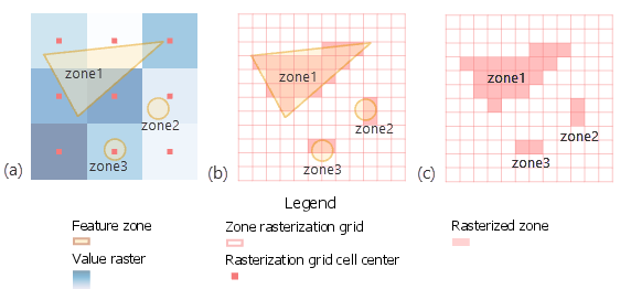
Just using the grid cell centers can result in a poor representation of the weather that overlaps each region, particularly when the regions are of a similar size to the grid cells. In this case, you need to determine how much each grid cell overlaps with each region (see Fig. 7).

There are different ways of doing this, but one is to use QGIS. Within QGIS, you can create a shapefile with a rectangle for each grid cell. Then intersect those with the region shapefile, producing a separate polygon for each region-by-grid cell combination. Then have QGIS compute the area of each of those regions: these will give you the portion of grid cells to use.

Fig. 7 See more here.

Matching geographical unit observations

It is often necessary to match names within two datasets with geographical unit observations. For example, a country’s statistics ministry may report values by administrative unit, but to find out the actual spatial extent of those units, you may need to use the GADM shapefiles.

Matching observations by name can be very time-consuming. These problems even exist at the level of countries, where, for example, North Korea is regularly listed as “Democratic People’s Republic of Korea”, “Korea, North”, and “Korea, Dem. Rep.”; and information is indiscriminately reported for isolated regions or sovereign states (Guadeloupe’s data may or may not be included in France). Reporting units may not correspond to standard administrative units at all, and you will need to aggregate or disaggregate regions to match between datasets. Here are some suggestions for solving this problem:

1. Try to perform all merging on abbreviation codes rather than names. At the level of countries, use ISO alpha-3 codes if possible.

2. Use string matching. However, in this case, you will need to inspect all of the matches to make sure that they are correct.

3. Construct “translation functions” for each dataset, which map the regional names in that dataset to a canonical list of region names. For example, choose the names in one dataset as a canonical list, and name the matching functions as <dataset>2canonical and canonical2<dataset2>.