Working with gridded data#
Gridded data#
Weather data is traditionally collected at weather stations. Weather stations are imperfect, unevenly distributed point sources of data whose raw output may not be suitable for economic and policy applications. Weather readings may be biased - for example, rain gauges tend to underestimate peak rainfall, and air temperature sensors often become more inaccurate at extreme temperatures.
Weather stations are more likely to be located in wealthier and more populated areas, which makes them less useful for work in developing countries or for non-human variables such as agriculture. Their number and coverage constantly change, making it difficult to compare across regions or time ranges. Despite being the most accurate tool for measuring the current weather at their location, they may hide microclimates nearby.
Thankfully, a large suite of data products has been developed to mitigate these issues. These generally consist of combining or ‘assimilating’ many data sources and analysis method into a ‘gridded dataset’ - the earth is divided into a latitude x longitude (x height) grid, and one value for a variable (temperature, precipitation, etc.) is provided at each gridpoint and timestep. These data products generally cover either the whole globe (or all global land), or are specialized to a certain region, and provide consistent coverage at each grid point location.
Note
Some variables, especially relating to hydrology, may be better suited to station data, by providing single values for large regions such as river basins.
However, since the world is not made up of grids (i.e., the world is not broken up into 50 x 50 km chunks, within which all weather conditions are identical), some processing has to be done even for historical “weather” data, and other limitations arise. For historical data, this processing is one of the sources of differences between data products, and for climate model output, the simulation of sub-grid processes is the greatest source of uncertainty between models.
Caution
Keep in mind that just because a dataset exists at a certain resolution does not mean it is accurate at that resolution!
The next section will briefly introduce how these products are generated, how to choose between them, and best practices for using “historical” data.
Gridded weather data products#
The Interpolation - Reanalysis Spectrum: Historical data products differ by how they “assimilate” (join observational with model data) or combine data, and how much “additional” information is added beyond (pre-processed) station data. They can be thought of as a rough spectrum ranging from ‘observational’ data products that merely statistically interpolate data into a grid to ‘reanalysis’ products that feed data products into a sort of climate model to produce a more complete set of variables. Some datasets are observational but include topographic and other physical information in their statistical methods, while some reanalysis datasets use pure model output for only some variables.
Both ends of their spectrum have tradeoffs, and generalizable statements about these tradeoffs are hard to make because of differences in methodologies. The following are a few simplified rules of thumb:
“Observational” / interpolated datasets#
Examples: GISTEMP, GHCN, Wilmot and Matsuura (aka “UDel”), Berkeley Earth (aka “BEST”), HadCrut4, PRISM, CHIRPS etc.
Observations (from weather stations, satellites, etc.) are statistically interpolated into a grid with little or no physical information added (though topography and - less commonly - wind speed are occasionally included)
Products generally differ by which stations or other data sources are included and excluded
Simple, biases well-understood
High correlation with source station data in areas with strong station coverage
Less realistic outside areas with strong station coverage
Statistical interpolation means data not bound by physicality
Often only available at lower temporal resolution (e.g., monthly)
See also
See also UCAR’s Model Data Guide summary on temperature datasets.
Reanalysis datasets#
Examples: ERA-INTERIM, ERA5, JRA-55, MERRA-2, NCEP2 (outdated), etc.
Observational data are combined with climate models to produce a full set of atmospheric variables
Products differ by what data is included (as with interpolated datasets), how that data is assimilated, but now also differ by which underlying models are used
Large extant literature on most major reanalysis products; limitations are generally well-understood (though not always well-estimated; and biases are often tested against interpolated datasets)
Coverage in areas with low station coverage (generally poorer or less populated areas) is more physically reasonable
Covers a large number of variables (though uncertainties differ between them)
Limited by often significant biases in underlying models that may or may not be well understood
Accuracy in areas of high station density may be lower than in interpolated products
Not fully physical either - laws of conservation, e.g., are often relaxed
See also
See also UCAR’s Model Data Guide summary on reanalyses.
Regional datasets#
Observational datasets exist with both global coverage (e.g., GISTEMP, HadCRUT, etc.) or regional coverage (e.g., PRISM in North America, TRMM in the tropics, etc.). Global datasets attempt to build a self-consistent database spanning the whole globe, and are therefore more likely to have sparser data coverage in specific regions - both as a logistical limitation, but also to ensure data pre-processing is as standardized as possible. Regional datasets may provide higher-resolution coverage and more specialized methodologies by incorporating local climatological knowledge or data sources that are not publicly available or parsable by global datasets (see e.g., the discussion in Dinku et al. 2019).
Satellite data#
Much of our observations for entire classes of variables (clouds, land surface characteristics such as NDVI, etc.), or over regions with sparse data coverage, comes from satellites. In their raw form, these data often are complex to work with; their spatiotemporal coverage is limited to when satellites pass overhead, their grids are often unconventional, and much preprocessing needs to be done to translate sensor outputs to usable data. When new satellites come online to replace older instruments, data need to be recalibrated, and spurious jumps may occur. However, oftentimes these data are pre-processed and assimilated into gridded datasets - for example, the CHIRPS rainfall dataset uses the TRMM satellite dataset as an input. Note that even for variables such as NDVI or cloud cover there are gridded datasets that have reprocessed satellite data to be consistent and gridded. If you really need access to raw satellite output, we recommend reaching out to atmopsheric or land researchers with experience working with these data.
Temporal and spatial homogeneity#
The number and locations of weather stations, the technologies used to collect data, and the methods for processing data change over time. The creators of gridded datasets will have chosen a strategy for dealing with these differences. Some datasets, such as the IMERG rainfall dataset, provide high resolution data but at the expense of an inhomogenous data record, by using all satellites they can get data from at a given time. Other datasets (such as the temperature uncertainty ensemble of GISTEMP) emphasize temporal homogeneity to better study long-term trends.
Next, we will get into how to choose and work with weather data products - but before that, we’d like to leave you with two warnings on using hydrological variables and using station data.
A Warning on hydrological variables (precipitation, humidity, etc.)#
Precipitation is a special beast. It is spatiotemporally highly heterogeneous (it can rain a lot in one place, and not rain at all on the other side of the hill, or an hour or a minute later) and difficult to measure accurately. Unfortunately, since rain (or lack thereof) can have tremendous impacts on humans, we often have to find ways to work with rain observations.
Unlike temperature, which is relatively uniform spatiotemporally and can be interpolated with a relatively high degree of confidence, precipitation data is very difficult to interpolate and requires a more sophisticated understanding of regional precipitation patterns to assimilate into gridded products. Consequently, gridded precipitation data should be used with “extreme caution”, and its uncertainties should not be underestimated.
Even ‘raw’ precipitation data from weather stations and rain gauges are problematic. Developing a reliable, easily scaled rain gauge network is a difficult task. For example, a common type of rain gauge, the ‘tipping bucket’, only records rain in discrete intervals (when the bucket fills and subsequently ‘tips’), and therefore could record a rainstorm if a drizzle tips an already-full bucket. In rare cases, tipping buckets stationed in remote areas may be stuck in the “tipped” position for some time before anyone notices or can repair them.

Fig. 3 “Hi, I’m your new meteorologist and a former software developer. Hey, when we say 12pm, does that mean the hour from 12pm to 1pm, or the hour centered on 12pm? Or is it a snapshot at 12:00 exactly? Because our 24-hour forecast has midnight at both ends, and I’m worried we have an off-by-one error.” - Several common dilemmas when using rain data#
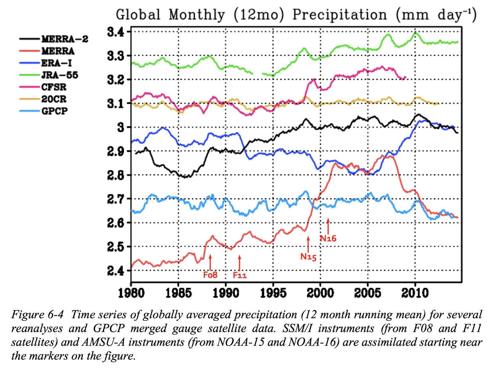
Fig. 4 Data from Bosilovich et al. (2015). Gridded data products disagree on average global monthly precipitation by up to 40%, and aren’t always consistent!#
In general, rain gauges of most types are biased low. In strong wind conditions, many drops may not enter the rain catch in a gauge due to turbulence; in strong storms, point estimates may miss areas of greatest intensity. Rain data averaged over areas with complex terrain is biased because of the vertical profile of precipitation (stations are generally in valleys). Kenji Matsuura (of the UDel dataset fame) in his expert guidance on his dataset explains: “Under-catch bias can be nontrivial and very difficult to estimate adequately, especially over extensive areas…”
Bias-correcting is integrated into weather data products, often involving assimilation of multiple data sources (satellites, radar, etc.) but significant biases remain (see above Figure).
Precipitation is often recommended as a control in economic models, but its unique character makes it difficult to work with. Beyond the strong uncertainty in precipitation data, precipitation is highly non-gaussian and its correlation with temperature is time- and space-dependent. When using precipitation in your model, be aware of its limitations, check robustness against multiple data products, or on geographic subsets that have better station coverage and potentially less biased data. Make sure to read studies evaluating your chosen data product - for example Dinku et al. 2018 for CHIRPS in Eastern Africa. Finally, make sure you think about what role precipitation plays in your model - see choosing weather variables!
Tip
A useful Google Scholar search for any product could be [data product name] validation OR evaluation OR bias OR uncertainty.
A warning on using station data#
Station data (e.g., Global Historical Climatology Network (GHCN) and the Global Summary of the Day) can be useful in policy and economic applications, and has been frequently used by especially older studies in the field. It provides a high degree of accuracy in areas of high station density, which generally corresponds to areas with a higher population density and a higher income level. Especially if you are working with urban areas, station data will likely capture the urban heat island effect more accurately than any gridded product.
However, station data can’t be seen as the ‘true’ weather either; assumptions and calibration methodologies affect data here as well (see e.g., Parker 2015), some variables remain rather uncertain, and the influence of microclimates even in close proximity to stations shouldn’t be underestimated (think for example the Greater Los Angeles region, where temperature can vary up to 35 F between the inland valleys and the coast).
Do not interpolate data yourself
Under normal circumstances, do not try to interpolate data yourself. Interpolated and reanalysis data products covered above were specifically designed for this purpose and have vetted methodologies and publicly available citable diagnostics and uncertainties.